A lot of teams land in Redshift the same way. Product events are flowing in, support data is getting centralized, dashboards look fine at first, and then one month later the core retention query starts dragging. The SQL didn't suddenly get worse. The table design did not keep up with the workload.

That matters most in product analytics because the query patterns are predictable and heavy. You filter by time, join events to users or accounts, aggregate by feature, and slice feedback by segment. If those tables were created with no thought beyond column names and data types, Redshift ends up doing extra work on every dashboard load and every ad hoc question.

Beyond Syntax Why Your Redshift Table Design Matters

When people first learn create table in Redshift, they often treat it like administrative setup. Define columns. Pick a few types. Load data. Move on. In practice, CREATE TABLE is where you decide how Redshift will physically lay out data for the next few million or few billion rows.

That's the part new analysts usually don't see yet. In an MPP warehouse, table design is query design. If a product dashboard joins user_events to users and accounts all day, your table layout affects whether Redshift can process that work cleanly in parallel or whether it has to shuffle data around first.

For product teams, this gets sharper because the workload is repetitive:

• Event analysis usually filters by timestamp and groups by user, account, or feature
• Feedback analysis often joins tickets or survey responses to account attributes
• Lifecycle reporting repeatedly asks for cohorts, active users, and conversion steps
• Self-serve exploration creates lots of similar scans with slightly different predicates

A decent logical model helps. If you need a quick refresher on how analytics tables usually separate measures from descriptive attributes, this fact and dimension tables guide is a useful companion before you start deciding on Redshift-specific physical design.

There's also a systems view here. If your warehouse schema is drifting because no one mapped how product data, billing data, and support data fit together, it's worth sketching that out before you create another table. A simple data architecture diagram workflow often catches bad joins and duplicate entities before they become warehouse problems.

Practical rule: If a dashboard is slow, don't start by blaming SQL syntax. Start by checking how the underlying tables were created.

Poor table design usually shows up as a pattern, not a single failure. Joins become inconsistent. Time-window queries scan too much data. Derived tables multiply because analysts stop trusting the base tables. The fix isn't magical. It's making better choices at table creation time, especially for distribution, sort order, and the shape of your analytics model.

The Two Core Methods to Create Tables in Redshift

There are two commands frequently used: CREATE TABLE and CREATE TABLE AS, usually shortened to CTAS. Both create tables, but they solve different problems.

Use CREATE TABLE when you need a durable schema

Use plain CREATE TABLE when you know the table definition up front and want control over data types, defaults, constraints, and physical design. This is the normal choice for core analytics tables like raw events, account snapshots, or curated feedback records.

Here's a practical example for a product analytics event table:

CREATE TABLE analytics.user_events (
    event_id BIGINT IDENTITY(1,1),
    event_timestamp TIMESTAMP NOT NULL,
    user_id BIGINT NOT NULL,
    account_id BIGINT,
    session_id VARCHAR(128),
    event_name VARCHAR(100) NOT NULL,
    page_name VARCHAR(255),
    feature_name VARCHAR(255),
    event_source VARCHAR(50),
    properties_json VARCHAR(65535),
    received_at TIMESTAMP DEFAULT GETDATE()
)
DISTSTYLE AUTO
SORTKEY AUTO;

This is a solid default starting point for a growing team because it keeps the schema explicit while letting Redshift make some physical-layout decisions automatically. You can get very far with this pattern if your workload is still evolving and you don't yet know which join path or filter pattern dominates.

A few practical notes:

• Use narrow types where you can. Don't make every ID a VARCHAR just because the source system did.
• Separate stable columns from messy payloads. Commonly queried fields like event_name or feature_name should be first-class columns, not buried in JSON text.
• Keep ingestion-friendly tables simple. Raw event tables should accept data cleanly. You can always build downstream marts with tighter semantics.

Use CTAS when you want to materialize a query result

CREATE TABLE AS is what you use when the table is the output of a transformation. It's ideal for summary tables, rollups, filtered subsets, and intermediate modeling steps.

For example, if product managers keep asking for daily active users, materialize that once and query the result directly:

CREATE TABLE analytics.daily_active_users AS
SELECT
    DATE_TRUNC('day', event_timestamp) AS activity_date,
    account_id,
    COUNT(DISTINCT user_id) AS dau
FROM analytics.user_events
WHERE event_name IN ('session_started', 'page_view', 'feature_used')
GROUP BY 1, 2;

This pattern is common in product analytics because the same aggregations get queried repeatedly. Instead of recalculating them in every BI query, you create a durable table that analysts and dashboards can hit directly.

CTAS is also useful when you want to:

• Reshape a wide raw table into a narrower analytics table
• Filter to a trusted subset such as production events only
• Precompute expensive aggregates for dashboards
• Stage transformations in ELT pipelines

A good CTAS table removes repeated work from every downstream query.

Temporary tables are for session-scoped work

Redshift also supports temporary tables. Use them for intermediate steps during analysis or transformations when the table doesn't need to persist after the session.

Example:

CREATE TEMP TABLE recent_trial_accounts AS
SELECT account_id, created_at
FROM analytics.accounts
WHERE plan_type = 'trial'
  AND created_at >= DATEADD(day, -30, GETDATE());

Temporary tables are useful for debugging a modeling step, breaking a complex query into pieces, or building a one-session enrichment before a final insert. They keep your permanent schema cleaner and reduce clutter in shared analytics environments.

The practical decision

A simple way to choose:

If the table represents a long-term business object, define it deliberately with CREATE TABLE. If it represents the result of a transformation, use CTAS. If it only helps you finish the current session's work, make it temporary.

Optimizing Performance with Distribution and Sort Keys

Most Redshift performance problems come down to one question. Where does the data live, and in what order is it stored?

Redshift is an MPP system. That means it spreads work across compute resources in parallel. If related rows are distributed sensibly and stored in a useful order, product analytics queries stay fast. If not, joins get expensive and scans get broader than they need to be.

A quick visual makes the trade-off easier to see.

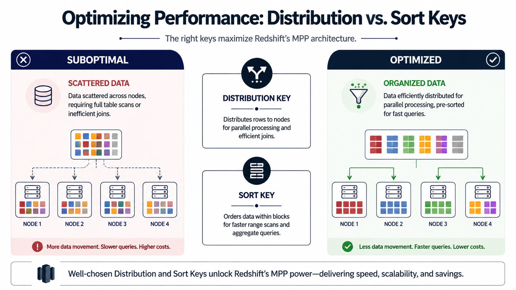
Distribution decides where rows go

Think of distribution like shelving books across several rooms. If books that are often referenced together are placed in the same room, the librarian works faster. If related books are scattered everywhere, every request turns into extra walking.

Redshift supports table-level options including DISTSTYLE {AUTO | EVEN | KEY | ALL}, DISTKEY(column_name), [COMPOUND | INTERLEAVED] SORTKEY(column_name, ...), and SORTKEY AUTO. AWS also notes that Redshift allows up to 400 sort key columns per table in the CREATE TABLE syntax documentation, which shows how much control teams can apply to physical layout for analytical workloads (AWS Redshift CREATE TABLE documentation).

Here's the practical comparison:

For product analytics, KEY often matters most on the big fact-style tables. If user_events and user_profiles are frequently joined on user_id, distributing both on user_id can reduce cross-node data movement during joins.

A practical version looks like this:

CREATE TABLE analytics.user_profiles (
    user_id BIGINT NOT NULL,
    account_id BIGINT,
    signup_date DATE,
    plan_tier VARCHAR(50),
    country_code VARCHAR(10)
)
DISTSTYLE KEY
DISTKEY (user_id)
COMPOUND SORTKEY (signup_date, user_id);

That design isn't universally right. It's right when the workload repeatedly joins on user_id. If most downstream analysis groups by account and rarely touches per-user joins, account_id might be the better choice. This is the trade-off. Pick the key that matches the dominant query path, not the one that feels conceptually neat.

Sort keys decide how Redshift reads the table

Distribution helps joins. Sort keys help scans.

If your analysts constantly ask questions like “What happened in the last 30 days?” or “Show feature usage this week by account segment,” sort order determines whether Redshift can skip irrelevant blocks or has to read much more of the table.

For event data, time is often the strongest candidate:

CREATE TABLE analytics.user_events_optimized (
    event_id BIGINT IDENTITY(1,1),
    event_timestamp TIMESTAMP NOT NULL,
    user_id BIGINT NOT NULL,
    account_id BIGINT,
    event_name VARCHAR(100) NOT NULL,
    feature_name VARCHAR(255)
)
DISTSTYLE KEY
DISTKEY (user_id)
COMPOUND SORTKEY (event_timestamp, user_id);

A compound sort key works best when queries usually filter from left to right. In product analytics, that's common. Teams usually start with a date or timestamp filter, then narrow by user, account, or event type.

An interleaved sort key can help when filtering happens across several columns with no clear priority, but it's usually a more specialized choice. For most event and behavioral models, compound sort keys are easier to reason about and align better with time-based analysis.

Later in the section, this walkthrough is worth watching if you want a more visual explanation of physical design trade-offs in Redshift:

What usually works for product teams

I'd keep the default decision path simple:

• **Start with ****DISTSTYLE AUTO** when you're still learning the workload.
• **Move to ****DISTSTYLE KEY** for large tables with a dominant join column.
• Use **DISTSTYLE ALL** sparingly for small lookup tables that nearly everything joins to.
• Make time the first sort key when the table is event-heavy and most filters are date based.
• **Use ****SORTKEY AUTO** if you want Redshift to handle more of the decision-making while the workload matures.

If a table powers time-series product reporting, a bad sort key hurts every analyst every day.

The mistake I see most often is choosing keys based on schema aesthetics instead of query behavior. A clean-looking DDL isn't the goal. Fast joins and efficient scans are.

Choosing Compression Encodings for Storage Efficiency

Compression is one of those Redshift topics that sounds like a storage concern but behaves like a query-performance concern too. Compressed data uses less space, but the bigger win for analytics teams is that Redshift often has to read less data from disk during scans.

That matters on large event and feedback tables. If your user_events table has wide text attributes, or your support-ticket model stores lots of repeated categorical fields, encoding choices can make the table cheaper to store and less expensive to query in practice.

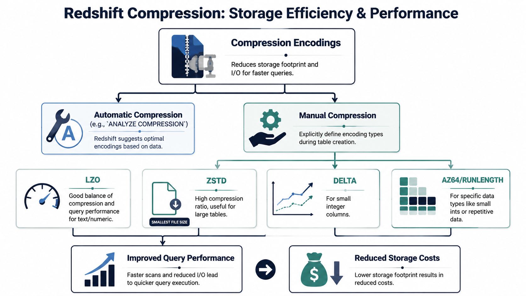
Default to automatic encoding first

A good starting point is to let Redshift handle compression automatically. That keeps you from prematurely hard-coding encodings before you understand real data distributions.

This is especially useful when product schemas evolve often. Event properties change. New support tags appear. Feedback pipelines expand. Automatic encoding keeps the initial DDL cleaner and avoids tuning work that may not survive the next model revision.

Know the common options anyway

You don't need to memorize every encoding, but it helps to recognize the usual families when you're tuning a large, stable table:

• **ZSTD** is commonly used for text-heavy columns and is a reasonable advanced option for large VARCHAR fields.
• **AZ64** is often associated with numeric and date-like columns.
• **LZO** is an older familiar option some teams still encounter in existing schemas.
• **BYTEDICT** can be relevant when a column has many repeated short values.

The lesson isn't “always use X.” It's that encoding should match column behavior. A free-form comment field and a low-cardinality status field don't compress the same way, and they shouldn't be treated the same way.

Where this hits product analytics

A product warehouse often stores two extremes together: narrow behavioral facts and bulky context fields. Think event_name beside properties_json, or ticket_status beside ticket_body. Compression helps balance those workloads so analysts can query broad fact sets without paying as much of a penalty for the text columns sitting next to them.

If you're also managing upstream object storage for raw exports, event archives, or unloaded staging files, this broader guide on DevOps-Strategien für S3-Kostenkontrolle is useful context for thinking about warehouse storage decisions alongside S3 cost hygiene.

Operational hint: Don't hand-tune encodings on day one unless you already know the table is critical, stable, and large.

The best return is typically achieved by focusing first on schema shape, distribution, and sort order. Compression is important, but it's usually the second or third optimization pass, not the first.

Post-Creation Maintenance and Verification

Creating the table is the launch. Keeping it healthy is the operating model.

In Redshift, that means you need a short checklist after table creation and after major load patterns change. Product analytics tables are especially prone to drift because they're loaded often, appended continuously, and sometimes updated by enrichment jobs that add account traits, classifications, or support metadata.

What Redshift now handles automatically

One of the better parts of modern Redshift is that stats management is much less manual than it used to be. AWS documents that ANALYZE updates statistical metadata used by the query planner, but in most cases you don't need to run it yourself because Redshift monitors workload changes and updates statistics in the background. AWS also states that COPY automatically analyzes an empty table, and Redshift analyzes new tables created with CREATE TABLE AS (CTAS) (AWS Redshift ANALYZE documentation).

That's a meaningful shift for data teams. Table creation, loading, and planner readiness are more integrated than they were in older warehouse operating models.

Still, automatic doesn't mean invisible. If a table changes substantially, or if certain columns drive joins, grouping, sorting, and predicates, explicit analysis can still be a sensible move.

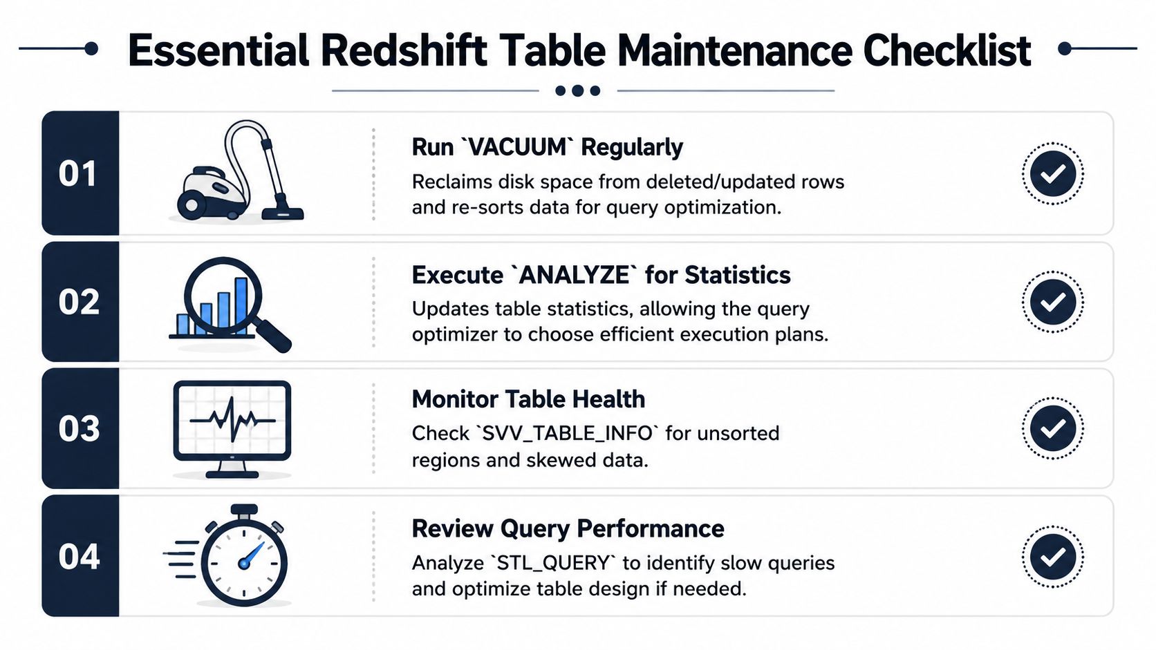
When manual maintenance is still worth it

VACUUM and ANALYZE shouldn't be run blindly on a schedule just because that was old warehouse folklore. They're tools for specific conditions.

Use manual attention when:

• Large deletes or updates happened and table organization may have degraded
• A major bulk load changed data distribution in a way the planner hasn't fully incorporated yet
• A key dashboard suddenly regressed and you need to rule out stale stats or poor sort health
• You changed the table's role from raw ingest storage to a heavily queried analytics object

For example:

VACUUM analytics.user_events;
ANALYZE analytics.user_events;

Those commands are most useful when there's a reason to expect disorder or stale planning inputs. They're not a substitute for good table design.

A healthy table is one whose physical design still matches the way analysts are querying it.

The verification checklist I'd run

After creating or materially changing a table, I'd verify a few things immediately:

SHOW TABLE analytics.user_events;

That confirms the effective DDL.

SELECT *
FROM svv_table_info
WHERE "table" = 'user_events';

That gives you a compact operational view of the table, including whether the sort state and distribution pattern still look healthy.

SELECT COUNT(*)
FROM analytics.user_events;

That's basic, but it catches load mistakes earlier than generally expected.

You can also review slow-query behavior in your monitoring workflow. If your team already thinks seriously about database observability, even outside Redshift, this expert guide to SQL Server monitoring is useful for the mindset. Different platform, same discipline: watch query behavior, validate assumptions, and don't wait for dashboards to become the alerting system.

Another practical check is data trust. A table that's physically optimized but semantically wrong is still a bad dependency for product reporting. Consequently, common data quality issues become tightly connected to warehouse maintenance. Duplicate IDs, inconsistent timestamps, and null-heavy join columns can make a well-designed Redshift table behave like a badly designed one.

A short post-launch habit

For any important new table, I'd do this after the first production load:

• Inspect the DDL so the created table matches the intended design
• **Check ****svv_table_info** for signs of skew or poor table health
• Validate row counts against the upstream expectation
• Run one representative query that mirrors the dashboard or model the table exists to support

That habit catches more issues than tuning after complaints arrive.

From Syntax to Strategy a Redshift Table Checklist

The teams that get value from Redshift fastest are not the ones who memorize the most syntax. They're the ones who treat create table in Redshift as a design decision tied to real workloads.

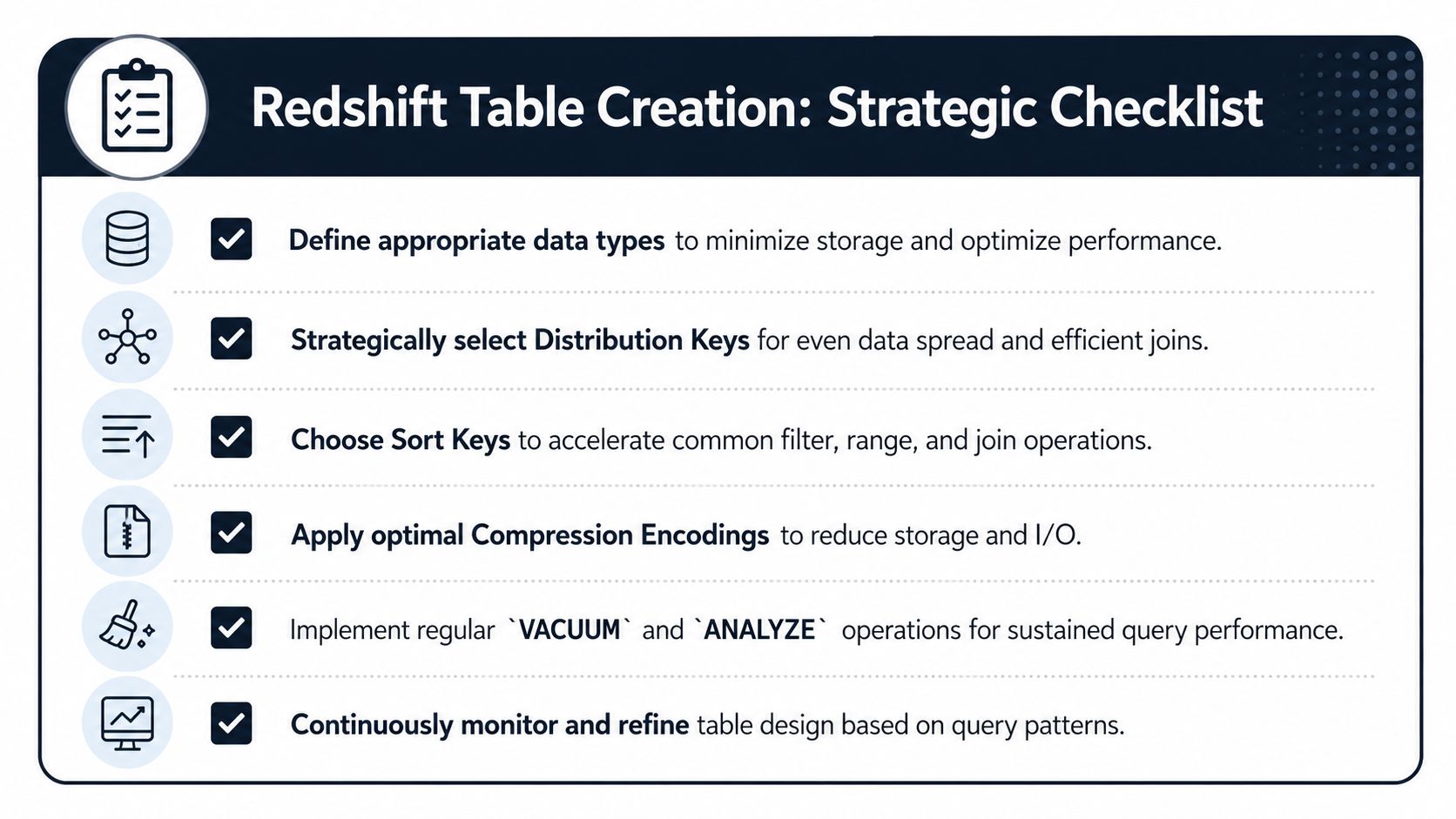
A practical checklist looks like this:

• Define columns for analytics use, not source-system convenience. Put frequently queried attributes in typed columns. Don't force every important field into JSON or giant text blobs.
• Pick distribution based on joins. If one key dominates joins across large tables, design for that behavior. If the workload is still unclear, let automation help first.
• Choose sort keys around filters. For most product event data, time is the first place to look because analysts usually ask time-bounded questions.
• Let automatic compression carry the initial load. Manual encoding is useful later, once the table is stable and important enough to justify deeper tuning.
• Verify after creation. A table isn't done when the DDL runs. Check how it was created, how it loaded, and whether it behaves the way the model expects.
• Design for self-serve use. If product managers and analysts will query the table directly, physical layout matters even more because query diversity goes up. A strong self-serve analytics approach yields significant returns.

The difference between a novice and a strong Redshift practitioner isn't syntax accuracy alone. It's recognizing that table design shapes cost, speed, and trust for every downstream question. That's especially true in product analytics, where the same joins and time filters show up every day.

If your team is trying to connect warehouse behavior with customer outcomes, SigOS helps product organizations turn support tickets, chat transcripts, sales calls, and usage patterns into prioritized signals. It's a useful next step when you've already built the data foundation and want clearer direction on which issues, requests, and behaviors matter most.